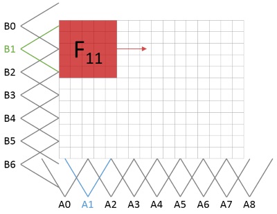
Goal
In this tutorial, the basic concept of fuzzy transform is presented. You will learn:
- mathematic background,
- how to apply concept of fuzziness to image processing.
The presented explanation demands knowledge of basic math. All related papers are cited and mostly accessible on https://www.researchgate.net/.
Introduction
In the last years, the theory of F-transforms has been intensively developed in many directions. In image processing, it has had successful applications in image compression and reduction, image fusion, edge detection and image reconstruction [Perf:FT] [MSLP:cod-decod] [Fusion:AFS12] [IPMU2012] [Perf:rec] [vlavsanek2015patch]. The F-transform is a technique that places a continuous/discrete function in correspondence with a finite vector of its F-transform components. In image processing, where images are identified by intensity functions of two arguments, the F-transform of the latter is given by a matrix of components.
Let me introduce F-transform of a 2D grayscale image \(I\) that is considered as a function \(I:[0,M]\times [0,N]\to [0,255]\) where \([0,M]=\{0,1,2,\ldots,M\}; [0,N]=\{0,1,2,\ldots,N\}\). It is assumed that the image is defined at points (pixels) that belong to the set \(P\), where \(P=\{(x,y)\mid x=0,1,\ldots, M;y=0,1,\ldots, N\}\).
Let \(A_0, \dots ,A_m\) and \(B_0, \dots ,B_n\) be basic functions, \(A_0, \dots ,A_m : [0,M] \to [0, 1]\) be fuzzy partition of \([0,M]\) and \(B_0, \dots ,B_n :[0,N]\to [0, 1]\) be fuzzy partition of \([0,N]\). Assume that the set of pixels \(P\) is sufficiently dense with respect to the chosen partitions. This means that for all \(k\in{0,\dots, m}(\exists x\in [0,M]) \ A_k(x)>0\), and for all \(l\in{0,\dots, n}(\exists y\in [0,N])\ B_l(y)>0\).
\(F^0\)
-transform
We say that the \(m\times n\)-matrix of real numbers \(F^0_{mn}[I] = (F^0_{kl})\) is called the (discrete) F-transform of \(I\) with respect to \(\{A_0, \dots,A_m\}\) and \(\{B_0, \dots,B_n\}\) if for all \(k=0,\dots,m,\ l=0,\dots,n\):
\[ F^0_{kl}=\frac{\sum_{y=0}^{N}\sum_{x=0}^{M} I(x,y)A_k(x)B_l(y)}{\sum_{y=0}^{N}\sum_{x=0}^{M} A_k(x)B_l(y)}. \]
The coefficients \(F^0_{kl}\) are called components of the \(F^0\)-transform.
\(F^1\)
-transform
\(F^1\)-transform has been presented in [perfilieva2014differentiation]. We say that matrix \(F^1_{mn}[I] = (F^1_{kl}), k=0,\ldots, m, l=0,\ldots, n\), is the \(F^1\)-transform of \(I\) with respect to \(\{A_k\times B_l\mid k=0,\ldots, m, l=0,\ldots, n\}\), and \(F^1_{kl}\) is the corresponding \(F^1\)-transform component.
The \(F^1\)-transform components of \(I\) are linear polynomials in the form
\[ F^1_{kl}(x,y)= c^{00}_{kl} + c^{10}_{kl}(x-x_k) + c^{01}_{kl}(y-y_l), \]
where the coefficients are given by
\[ c_{kl}^{00} =\frac{\sum_{y=0}^{N}\sum_{x=0}^{M} I(x,y)A_k(x)B_l(y)}{\sum_{y=0}^{N}\sum_{x=0}^{M} A_k(x)B_l(y)}, \\ c_{kl}^{10} =\frac{\sum_{y=0}^{N}\sum_{x=0}^{M} I(x,y)(x - x_k)A_k(x)B_l(y)}{\sum_{y=0}^{N}\sum_{x=0}^{M} (x - x_k)^2A_k(x)B_l(y)}, \\ c_{kl}^{01} =\frac{\sum_{y=0}^{N}\sum_{x=0}^{M} I(x,y)(y - y_l)A_k(x)B_l(y)}{\sum_{y=0}^{N}\sum_{x=0}^{M} (y - y_l)^2A_k(x)B_l(y)}. \]
Application to image processing
The technique of F-transforms uses two steps: direct and inverse. The direct step is described in the previous section whereas the inverse is as follows
\[ O(x,y)=\sum_{k=0}^{m}\sum_{l=0}^{n} F^d_{kl}A_k(x)B_l(y), \]
where \(O\) is the output (reconstructed) image and \(d\) is F-transform degree. In fact, the algorithm computes the F-transform components of the input image \(I\) and spreads the components afterwards to the size of \(I\). For details see [Perf:rec]. Application to image processing is possible to take from two different views.
From pixel point of view
The pixels are processed one by one in a way that appropriate basic functions are found for each of them. It will be exactly four, two in each direction. We need some helper structure in the memory for collecting their values. The values will be used in the nominator of the related fuzzy component. Implementation of this approach uses keyword FL as fast processing (because of more optimizations) and linear basic function.
From fuzzy component point of view
In this way, image is divided to the regular areas. Each area is processed separately using kernel window. This approach benefits from easy to understand, matrix based processing with straight forward parallelization.

This approach uses kernel \(g\). Let us show linear case with radius \(h = 2\) as an example.
\[ A = (0, 0.5, 1, 0.5, 0) \\ B^T = (0, 0.5, 1, 0.5, 0) \\ g = AB^T=\left( \begin{array}{ccccc} 0 & 0 & 0 & 0 & 0 \\ 0 & 0.25 & 0.5 & 0.25 & 0 \\ 0 & 0.5 & 1 & 0.5 & 0 \\ 0 & 0.25 & 0.5 & 0.25 & 0 \\ 0 & 0 & 0 & 0 & 0 \\ \end{array} \right) \]
 1.9.6
1.9.6