Table of Contents
Prev Tutorial: Object detection with Generalized Ballard and Guil Hough Transform
Next Tutorial: Affine Transformations
| Original author | Ana Huamán |
| Compatibility | OpenCV >= 3.0 |
Goal
In this tutorial you will learn how to:
a. Use the OpenCV function cv::remap to implement simple remapping routines.
Theory
What is remapping?
- It is the process of taking pixels from one place in the image and locating them in another position in a new image.
- To accomplish the mapping process, it might be necessary to do some interpolation for non-integer pixel locations, since there will not always be a one-to-one-pixel correspondence between source and destination images.
We can express the remap for every pixel location \((x,y)\) as:
\[g(x,y) = f ( h(x,y) )\]
where \(g()\) is the remapped image, \(f()\) the source image and \(h(x,y)\) is the mapping function that operates on \((x,y)\).
Let's think in a quick example. Imagine that we have an image \(I\) and, say, we want to do a remap such that:
\[h(x,y) = (I.cols - x, y )\]
What would happen? It is easily seen that the image would flip in the \(x\) direction. For instance, consider the input image:
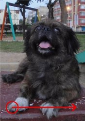
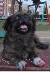
observe how the red circle changes positions with respect to x (considering \(x\) the horizontal direction):
- In OpenCV, the function cv::remap offers a simple remapping implementation.
Code
- What does this program do?
- Loads an image
- Each second, apply 1 of 4 different remapping processes to the image and display them indefinitely in a window.
- Wait for the user to exit the program
Explanation
Load an image:
Create the destination image and the two mapping matrices (for x and y )
Create a window to display results
Establish a loop. Each 1000 ms we update our mapping matrices (mat_x and mat_y) and apply them to our source image:
The function that applies the remapping is cv::remap . We give the following arguments:
- src: Source image
- dst: Destination image of same size as src
- map_x: The mapping function in the x direction. It is equivalent to the first component of \(h(i,j)\)
- map_y: Same as above, but in y direction. Note that map_y and map_x are both of the same size as src
- INTER_LINEAR: The type of interpolation to use for non-integer pixels. This is by default.
- BORDER_CONSTANT: Default
How do we update our mapping matrices mat_x and mat_y? Go on reading:
- Updating the mapping matrices: We are going to perform 4 different mappings:
- Reduce the picture to half its size and will display it in the middle:
\[h(i,j) = ( 2 \times i - src.cols/2 + 0.5, 2 \times j - src.rows/2 + 0.5)\]
for all pairs \((i,j)\) such that: \(\dfrac{src.cols}{4}<i<\dfrac{3 \cdot src.cols}{4}\) and \(\dfrac{src.rows}{4}<j<\dfrac{3 \cdot src.rows}{4}\) - Turn the image upside down: \(h( i, j ) = (i, src.rows - j)\)
- Reflect the image from left to right: \(h(i,j) = ( src.cols - i, j )\)
- Combination of b and c: \(h(i,j) = ( src.cols - i, src.rows - j )\)
- Reduce the picture to half its size and will display it in the middle:
This is expressed in the following snippet. Here, map_x represents the first coordinate of h(i,j) and map_y the second coordinate.
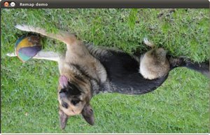
Result
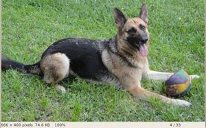
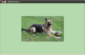
- After compiling the code above, you can execute it giving as argument an image path. For instance, by using the following image:
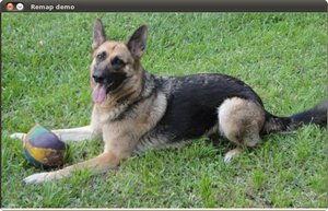
- This is the result of reducing it to half the size and centering it:
- Turning it upside down:
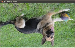
- Reflecting it in the x direction:
- Reflecting it in both directions: